

Intelligent ClinlAbomics Research Expedition
A modular R framework that takes clinical / omics data all the way from
raw table to publication-ready figures: statistics and missing-data
handling, feature selection, machine-learning benchmarking, unsupervised
subtyping (K-means, NMF, latent profile analysis), and prognostic /
survival modeling — each with an interactive Shiny deployment layer.





Maintainer: Huaichao Luo (luohc@uestc.edu.cn) —
Google Scholar |
ResearchGate |
Lab Twitter/X
Contributor: Guangchuang Yu — Lab website (yulab-smu.top)
📖 Full tutorial & documentation: yulab-smu.top/icare
- Overview
- See icare in action
- Installation
- The four modules
- Essential Commands
- Module 1 — Data cleaning (
Stat) - Module 2 — Modeling (
Train_Model) - Module 3 — Subtyping (
Subtyping) - Module 4 — Survival / Prognosis (
PrognosiX) - Quick start
- Getting help
- Citation
- License
icare organizes an analysis as a pipeline of S4 objects, one per stage,
each produced by converting the previous one with ConvertObject():
raw data.frame
      │  CreateStatObject()
      ▼
  Stat object  ──────────────► baseline table, group comparisons, DEG
      │  ConvertObject(to = "Train_Model")   ConvertObject(to = "Subtyping")   Stat_to_PrognosiX()
      ▼                                    ▼                                ▼
Train_Model object                 Subtyping object                PrognosiX object
(classification /                  (K-means / NMF / LPA)            (Cox / RSF / mlr3proba
 regression, caret)                                                  survival learners)
      │                                    │                                │
      ▼                                    ▼                                ▼
 ModelDeployment()                 New_Sub_Manager()               New_Prog_Manager()
      │                                    │                                │
      ▼                                    ▼                                ▼
deploy_clinlab_app()             launch_sub_deploy_app()          launch_prog_deploy_app()
Every stage keeps a record of what was done to the data (imputation
values, scaling parameters, selected features, trained models) inside the
object itself, so the exact same transformation can be replayed on new
patients at prediction time.
Real output from the QUICKSTART vignettes on real clinical/omics data — click any figure to open the full walkthrough that produced it. The example dataset used throughout Modules 1, 2,3, and 4 ships with the package at icare/inst/extdata/PMID37633276_DIA_plasmaproomic.xlsx.
|
Module 1 · Data cleaning & exploration Group-wise distributions and PCA ordination, straight out of |
Module 2 · Classification modeling
|
|
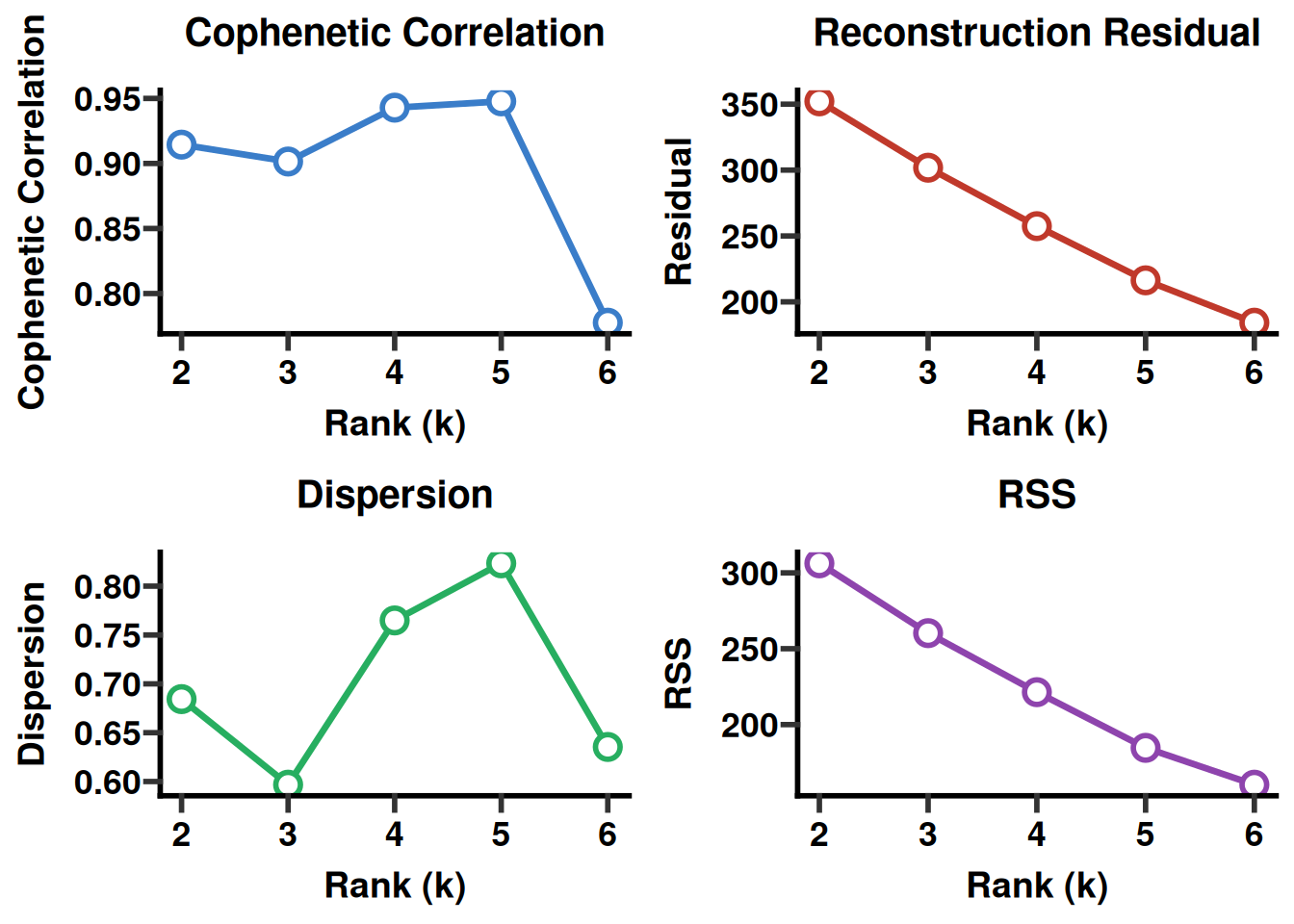
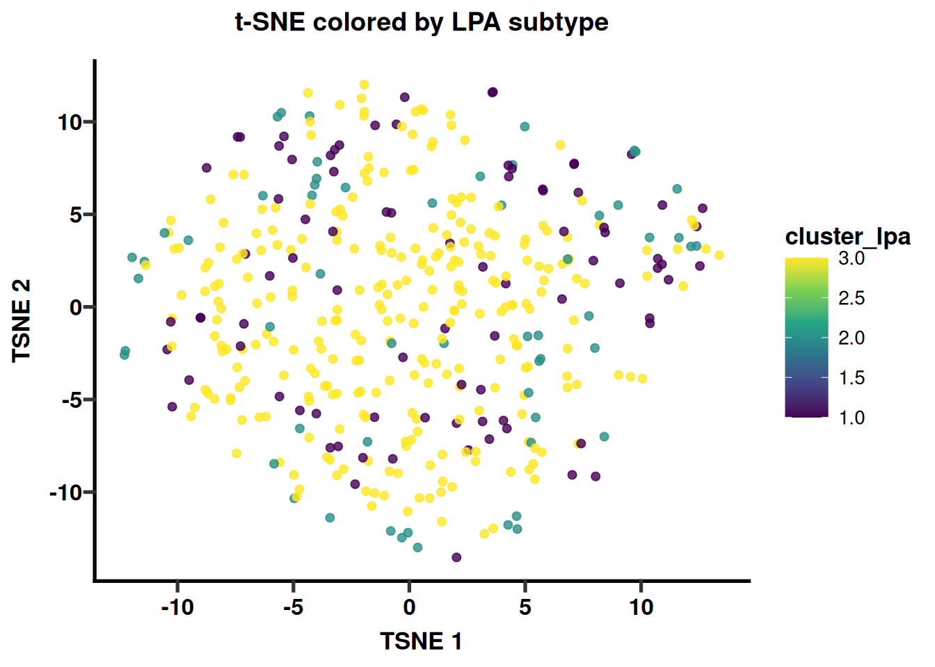
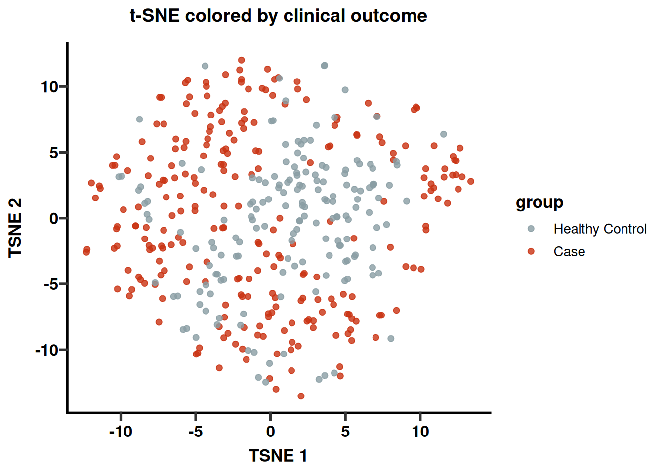
Module 3 · Unsupervised subtyping NMF rank estimation and the resulting t-SNE embedding, colored by subtype. → Quick-start chapter |
Module 4 · Survival & prognosis Median-split Kaplan–Meier curves from |
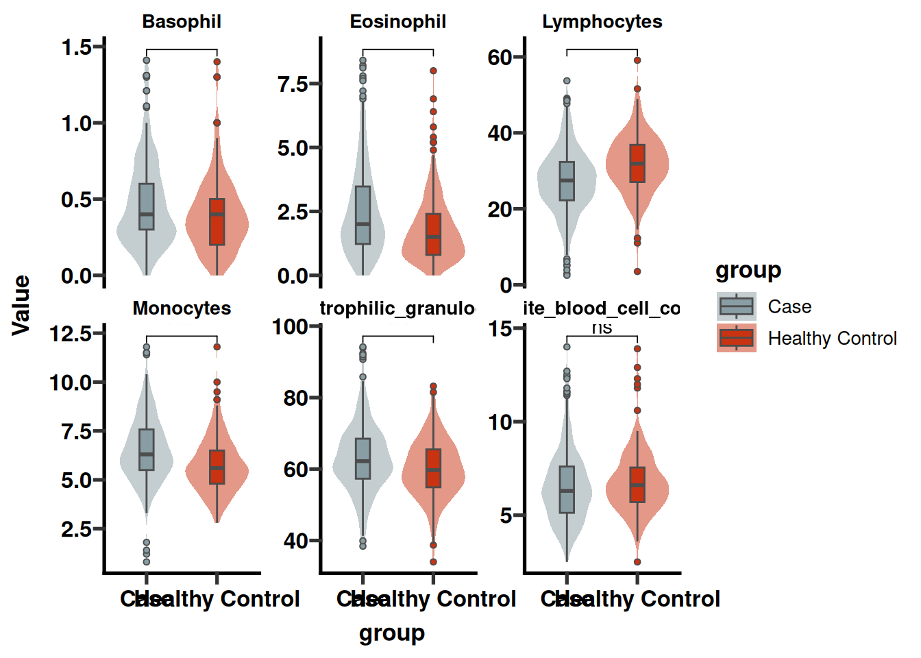
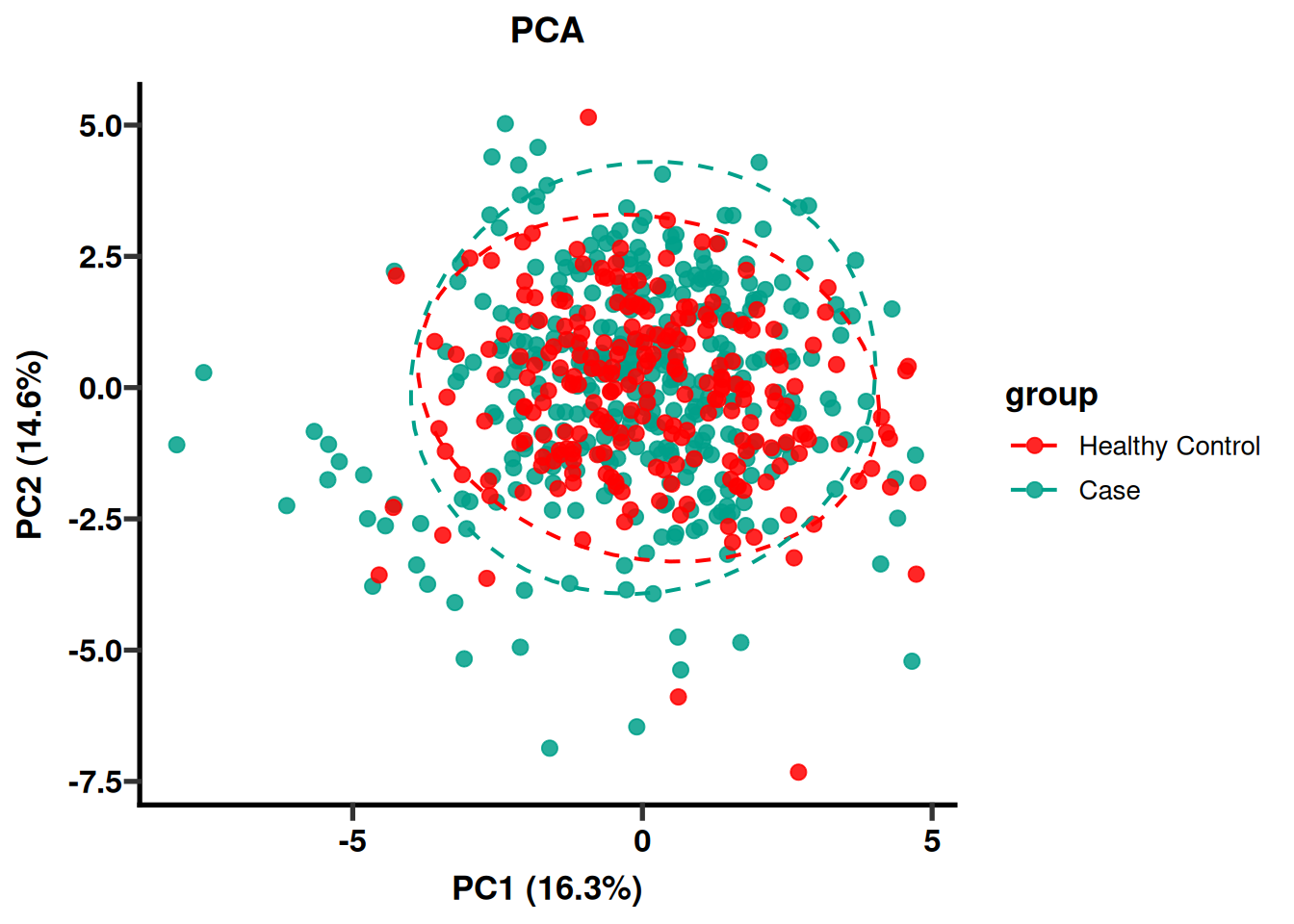
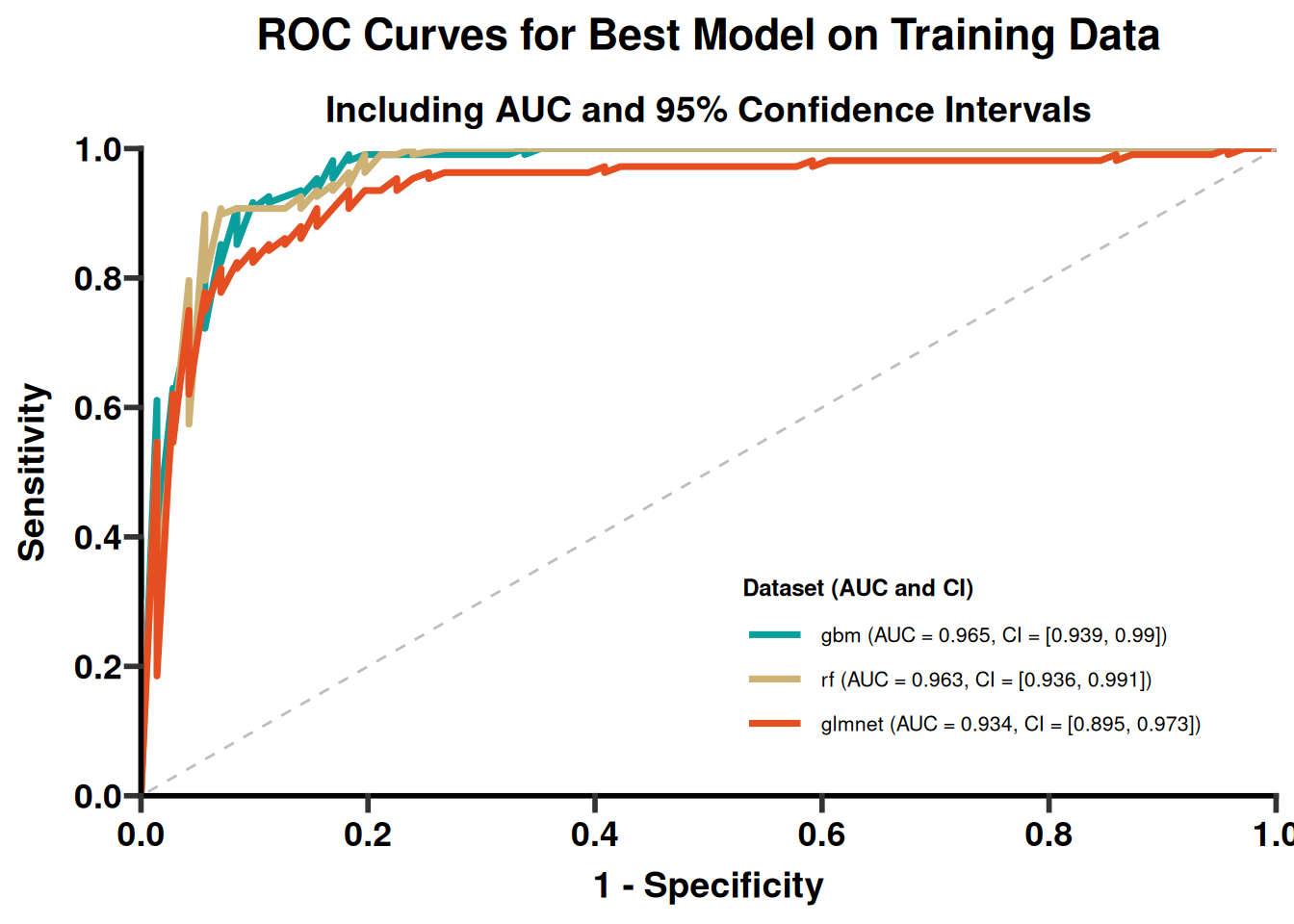
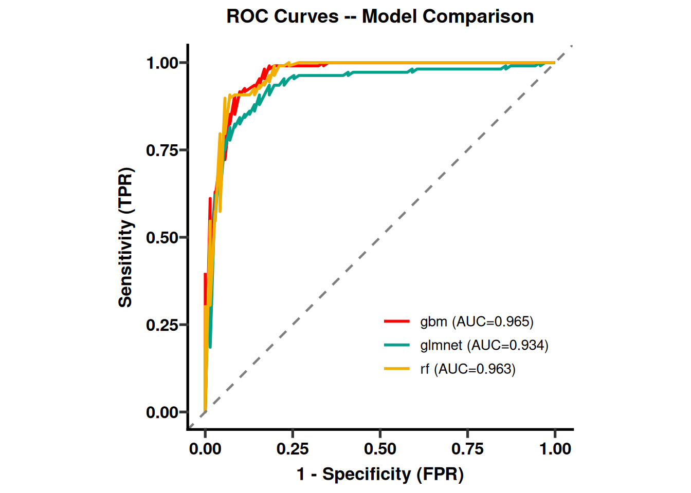
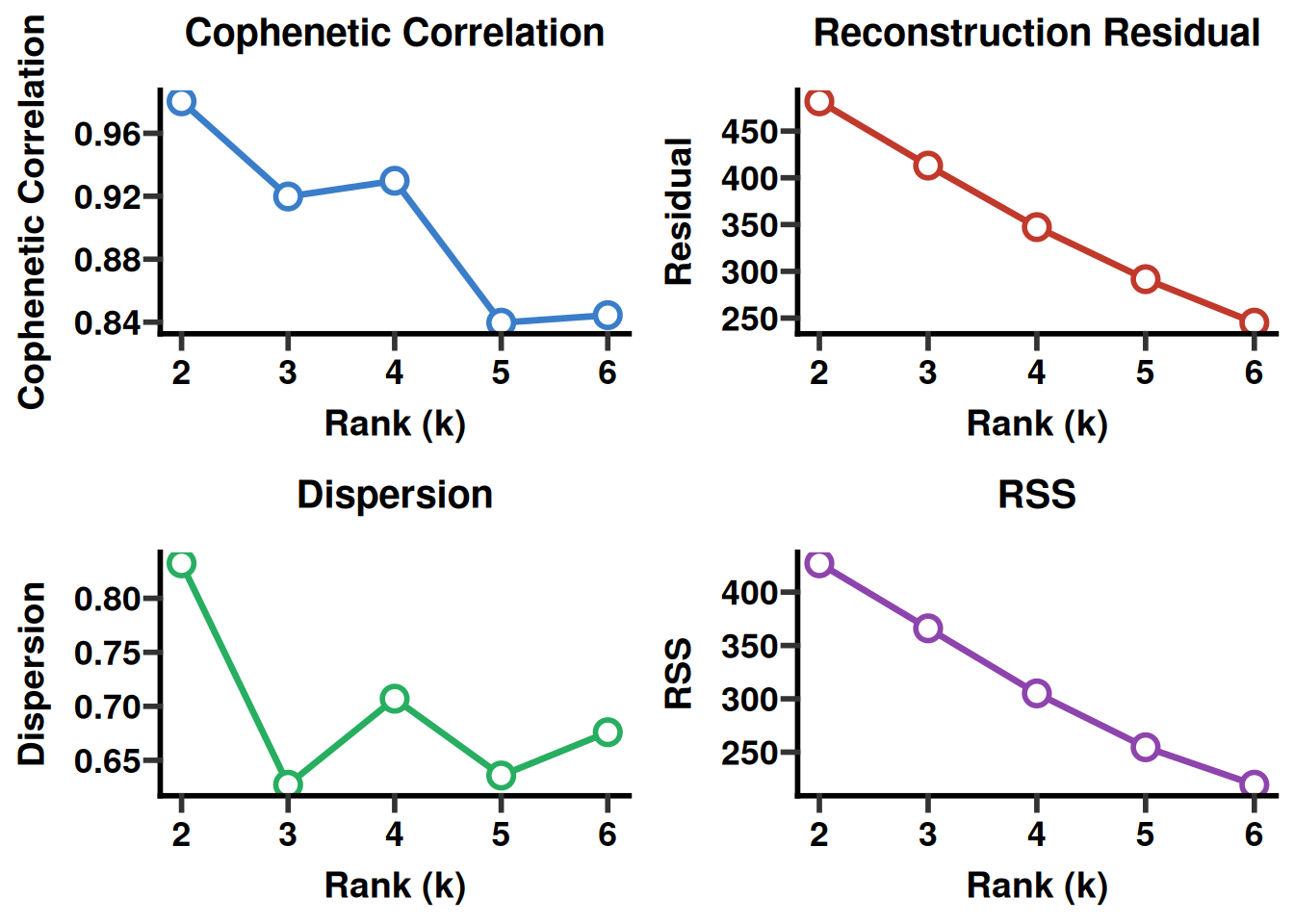
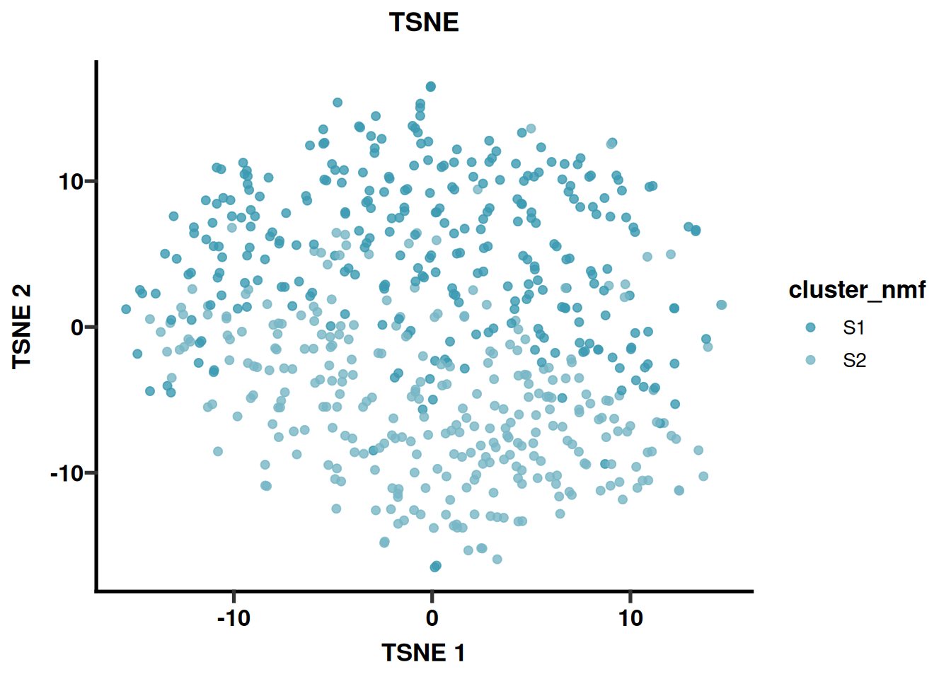
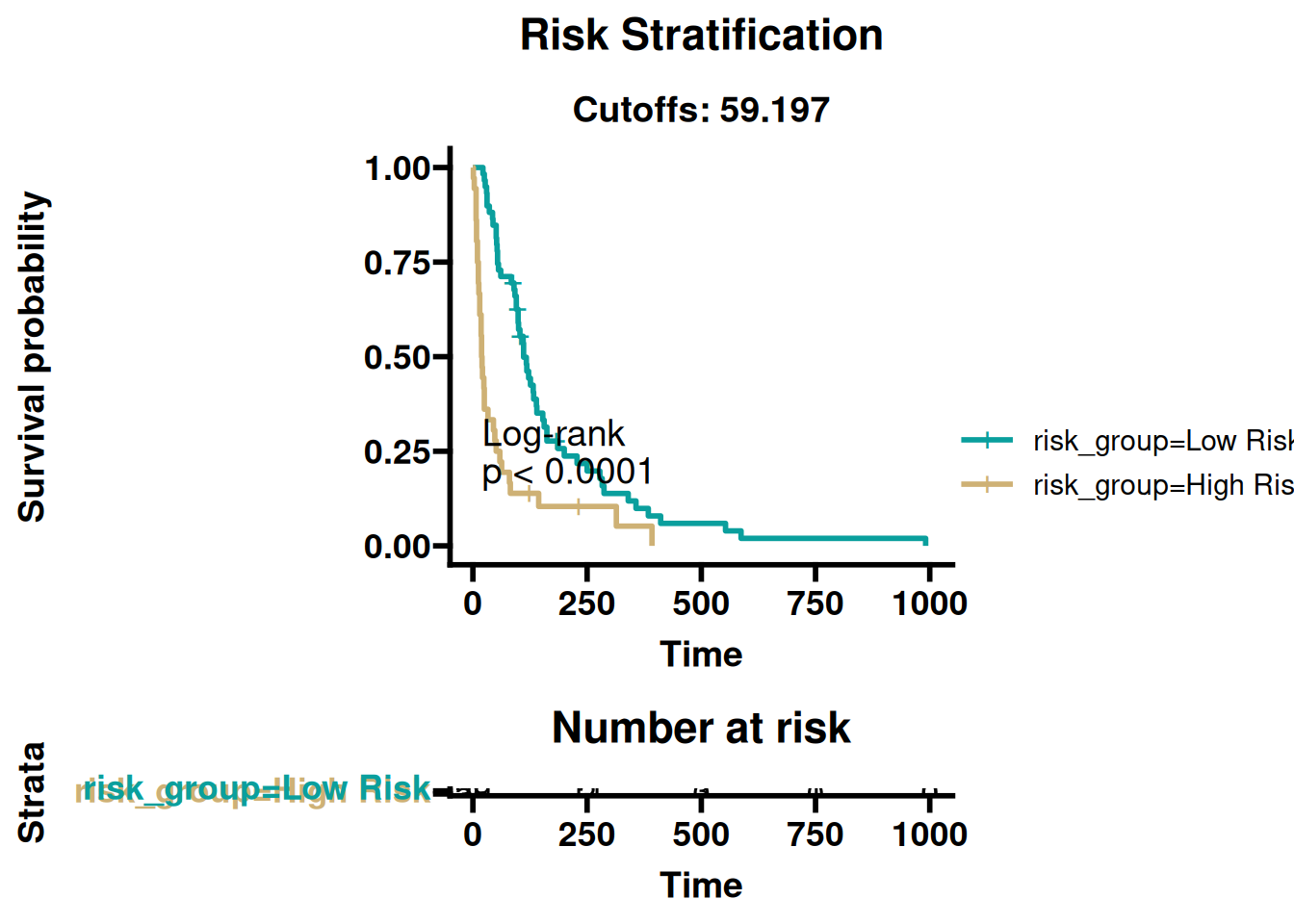
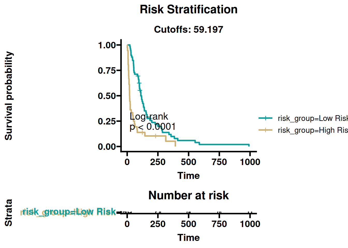
👉 Every chapter above (and their ADVANCED counterparts) is runnable end-to-end in the online book — code, console output, and figures are shown together, chunk by chunk.
The QUICKSTART chapters get you a result in minutes — the ADVANCED chapters are where icare earns its keep for a manuscript: multi-method feature selection with consensus/stability diagnostics, algorithm benchmarking with SHAP/DALEX explanations, three-way clustering validation, and full survival-model robustness/DCA/nomogram workflows. A taste of what each one produces:
|
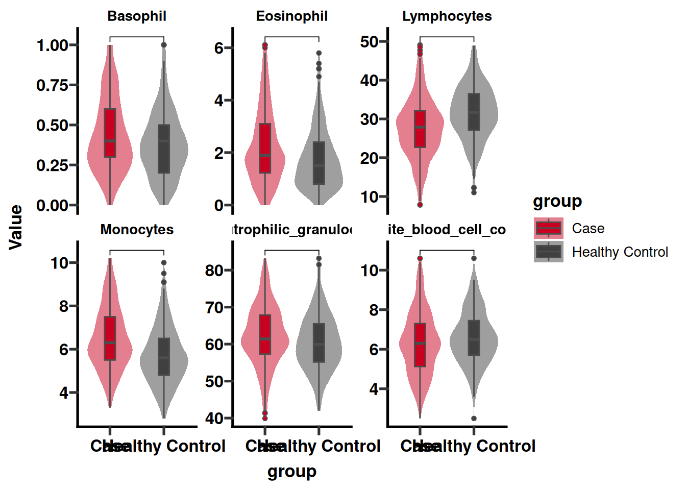
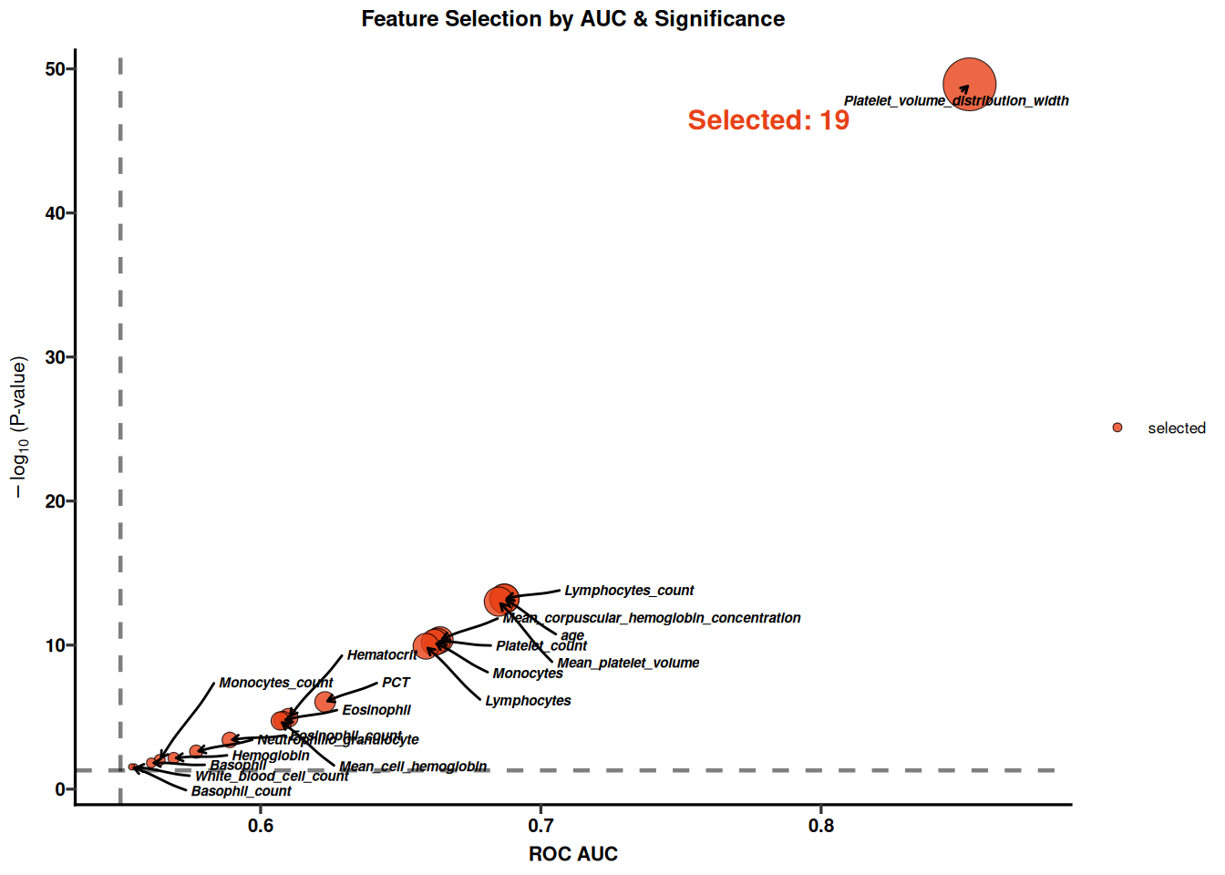
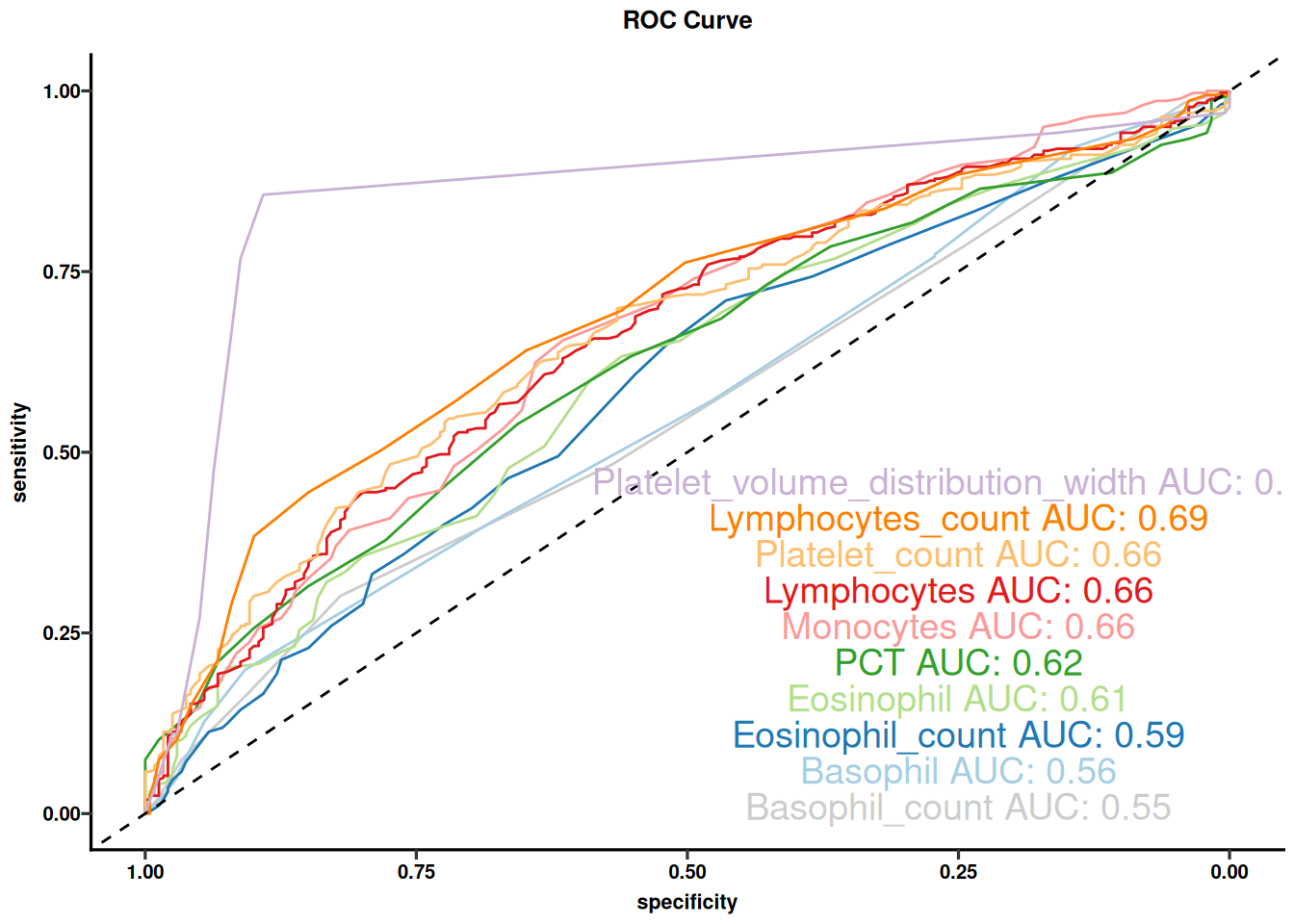
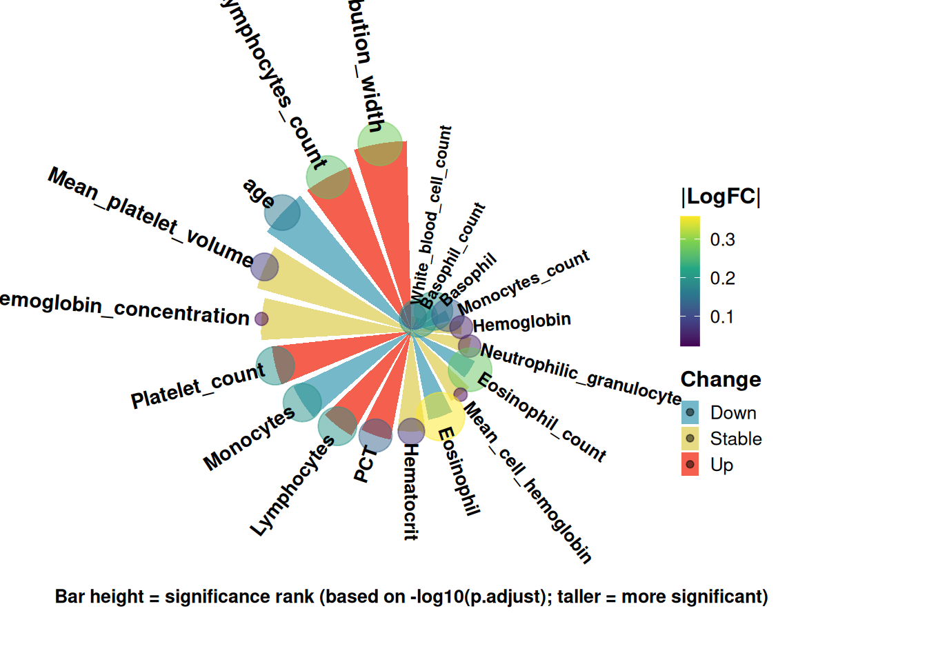
Module 1 · Advanced — publication figures Annotated PCA, AUC/p-value feature triage, annotated heatmaps, per-feature ROCs, radar charts, and a manuscript-ready "Table 1" — all in one script. → Advanced chapter |
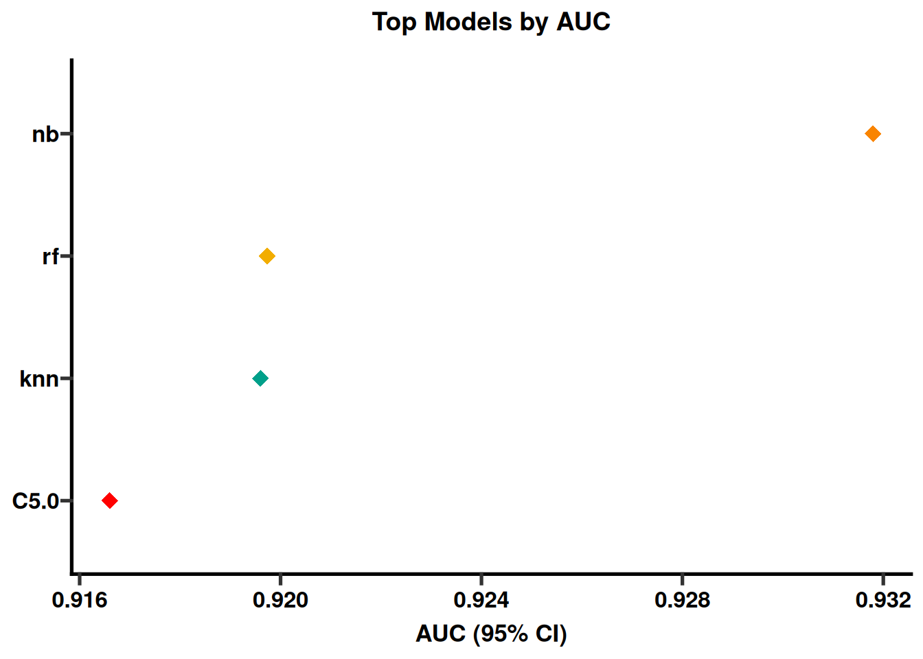
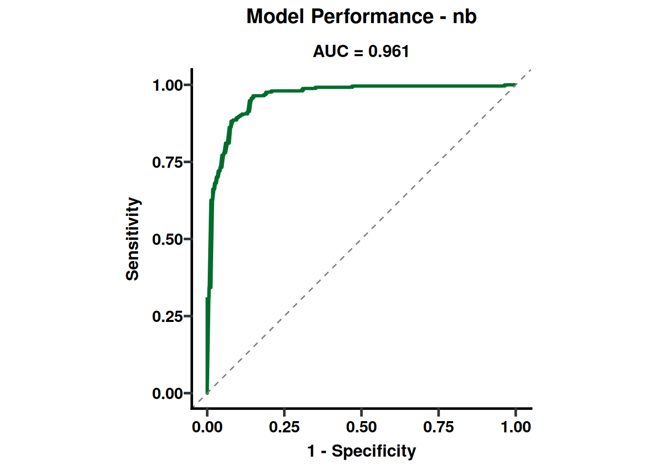
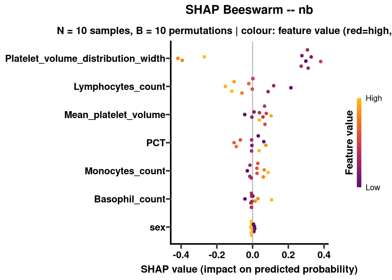
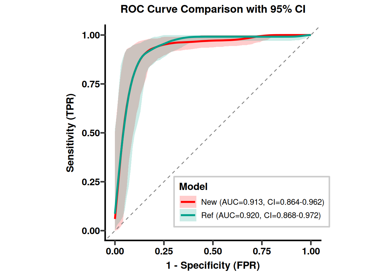
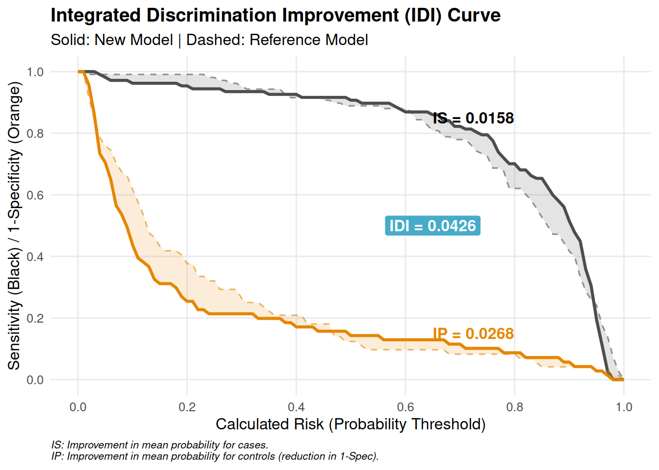
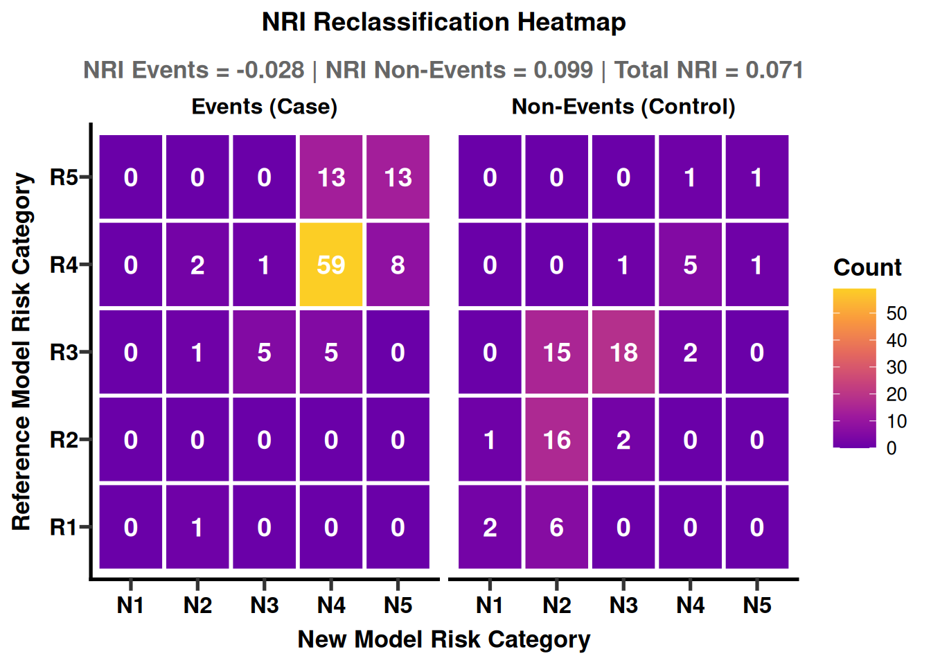
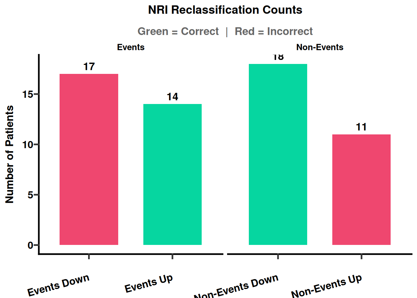
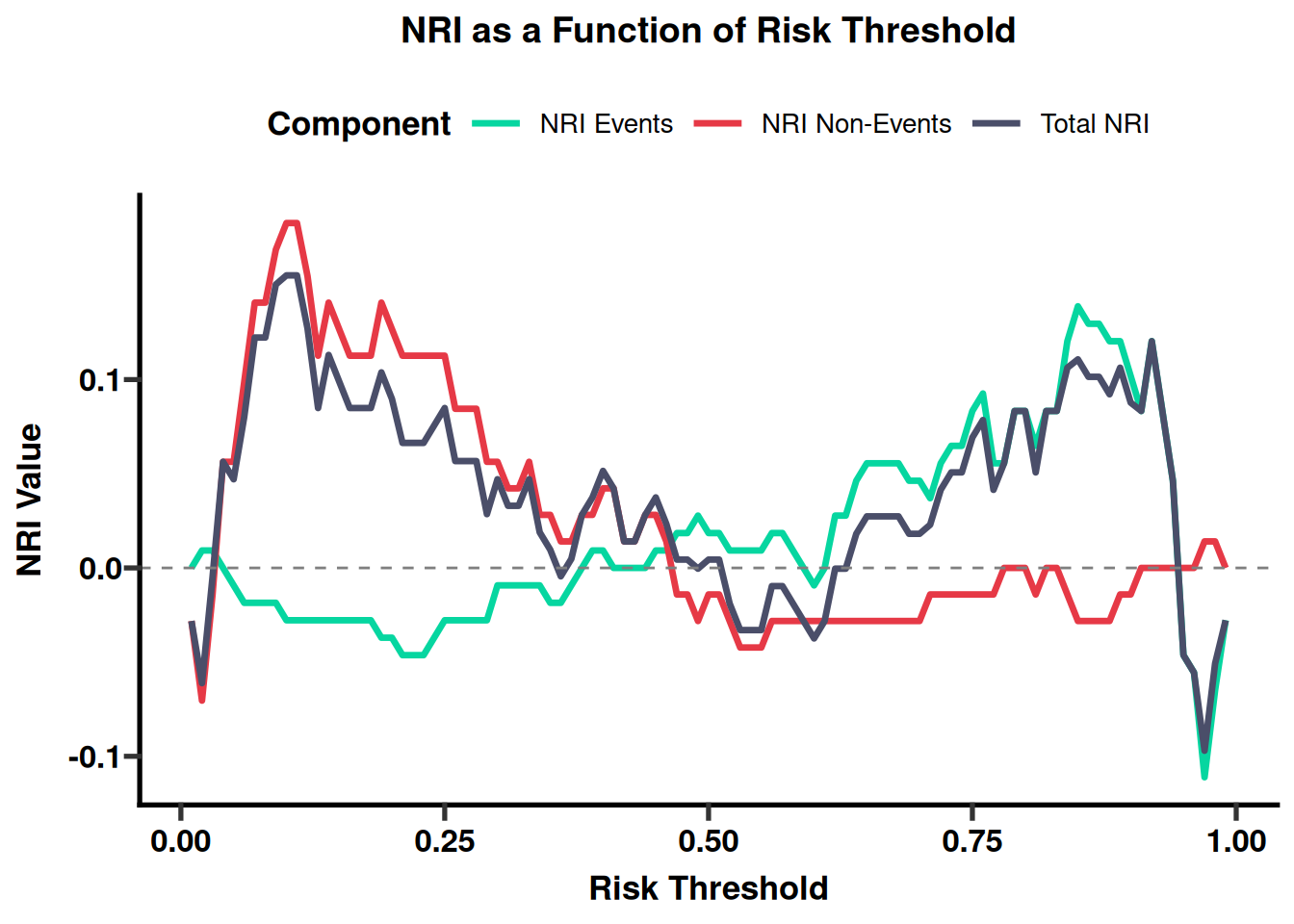
Module 2 · Advanced — benchmarking & explainability RFE/GA/SA consensus feature selection, a 9-algorithm benchmark, ensembling, Bayesian tuning, SHAP/DALEX explanations, decision thresholds, and NRI/IDI reclassification analysis. → Advanced chapter |
|
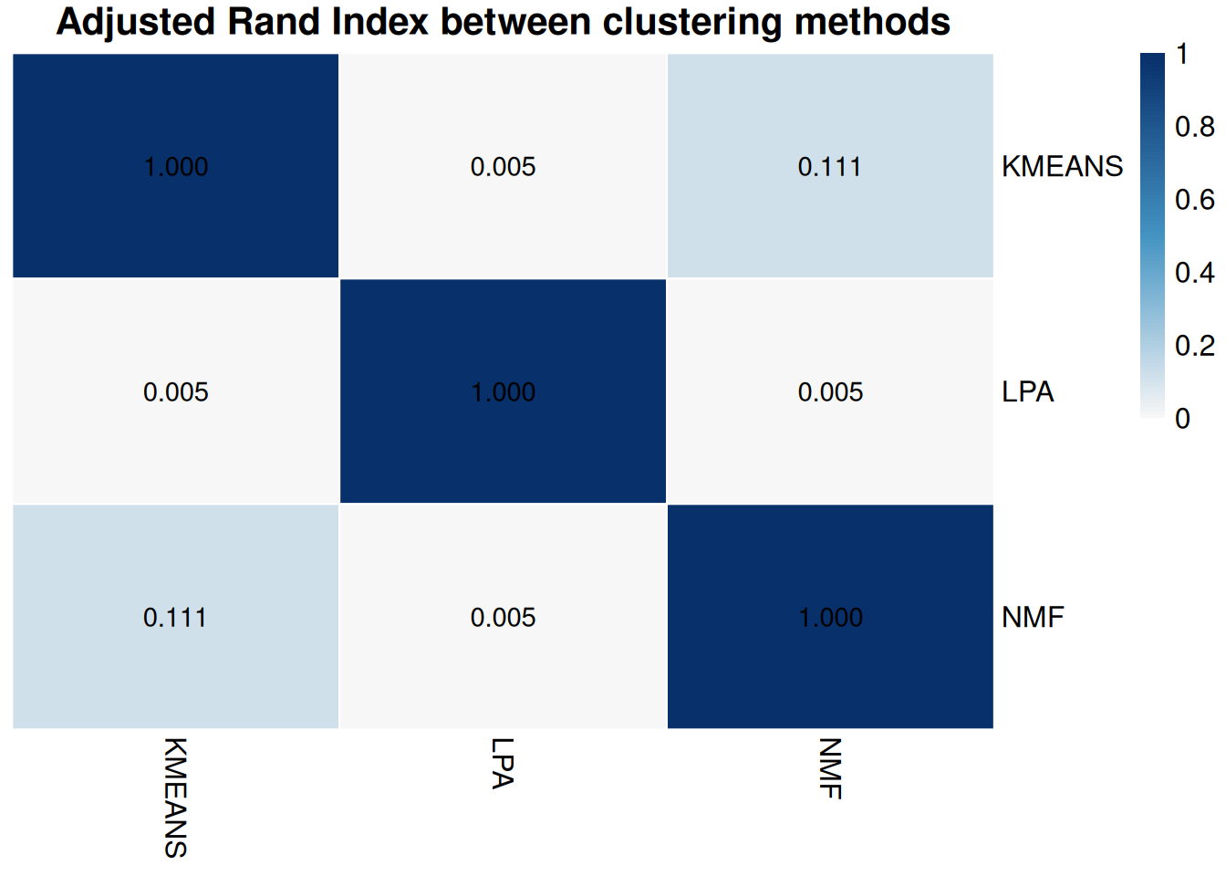
Module 3 · Advanced — three-way clustering validation K-means, LPA, and NMF cross-validated against each other (Adjusted Rand Index), with marker heatmaps, silhouettes, and an alluvial agreement diagram. → Advanced chapter |
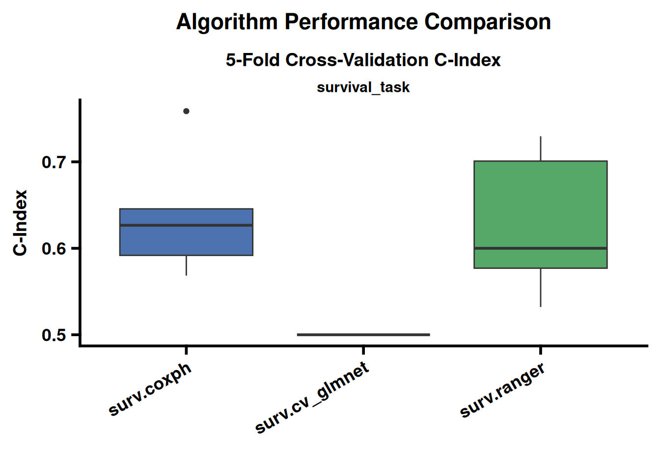
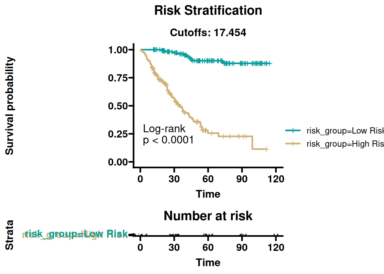
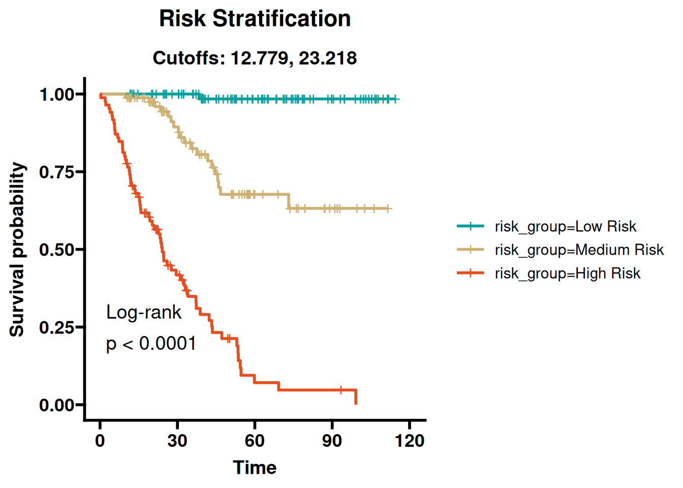
Module 4 · Advanced — robust survival modeling Strict train/validation split, algorithm benchmarking, subgroup forests, time-dependent AUC, calibration, nomograms, stability/ablation checks, DCA, and survival SHAP. → Advanced chapter |
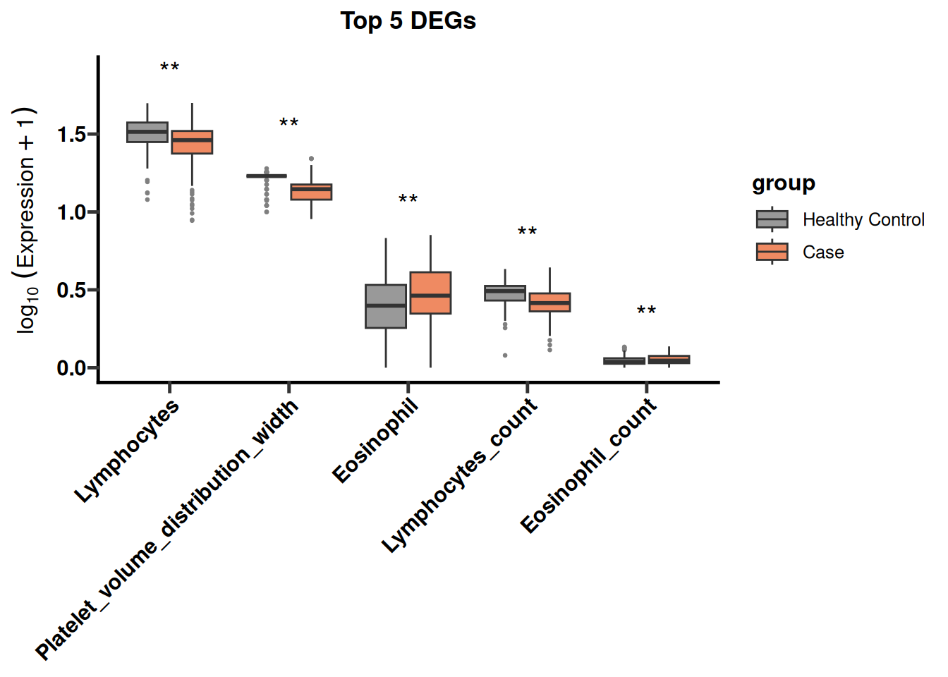
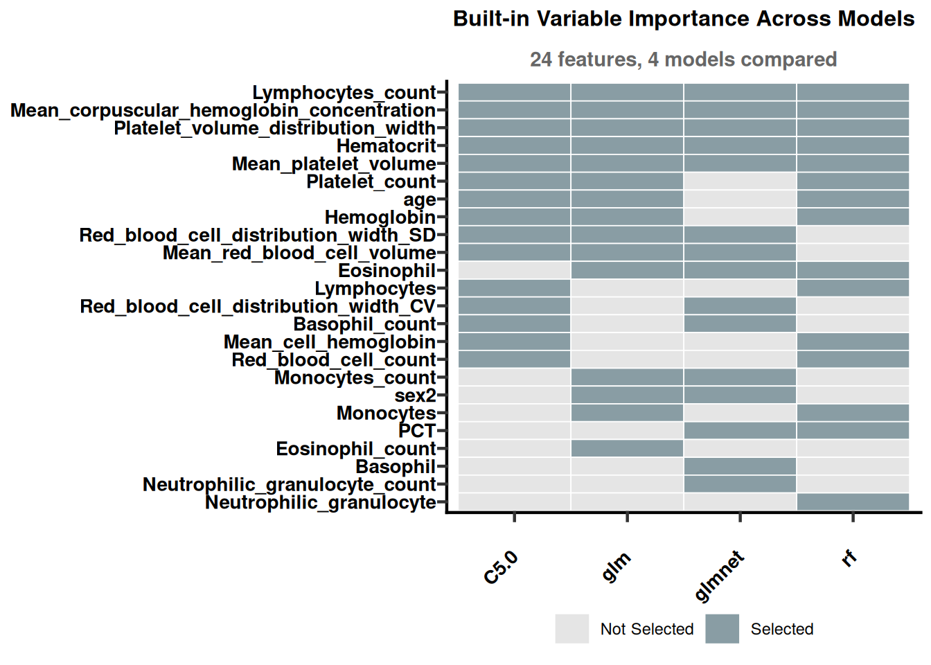
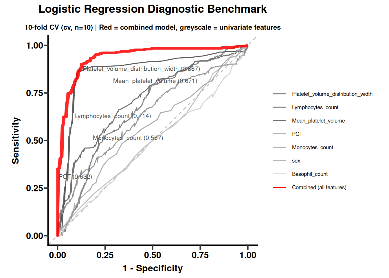
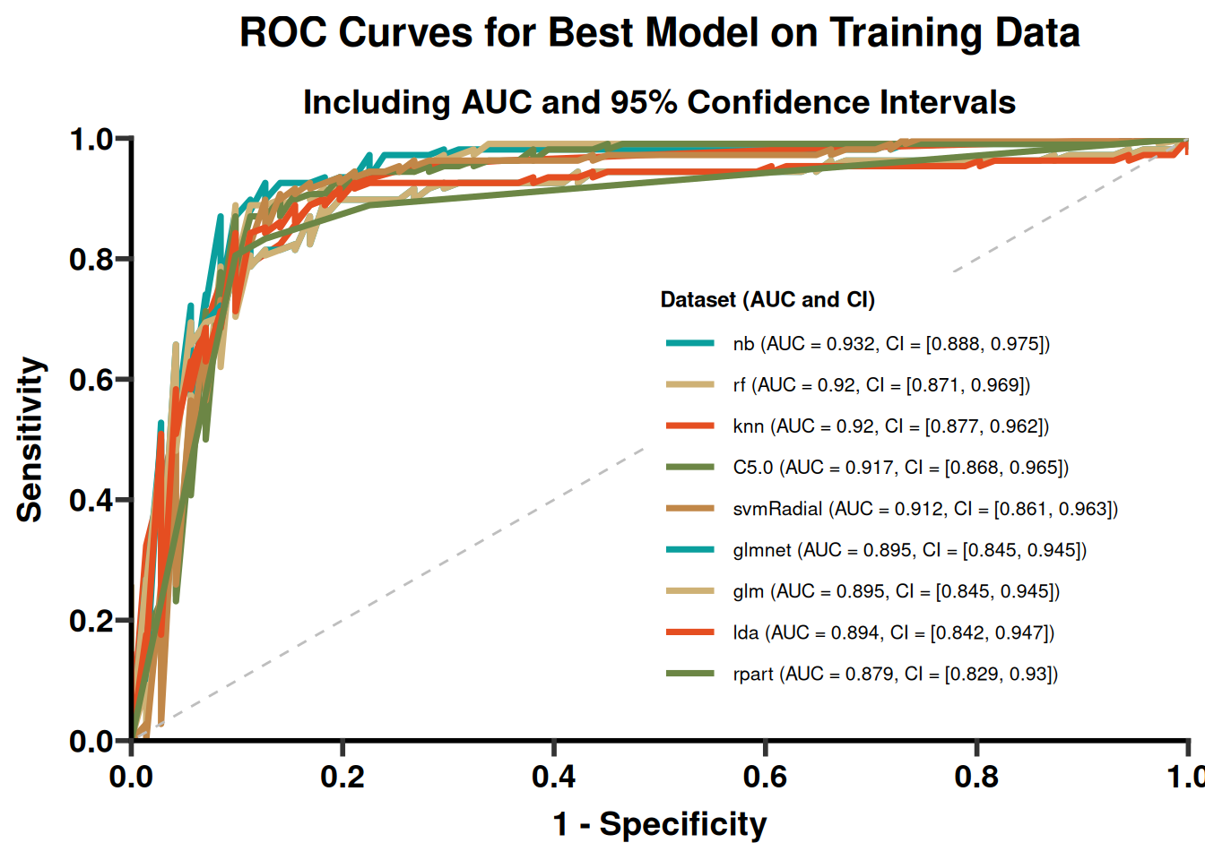
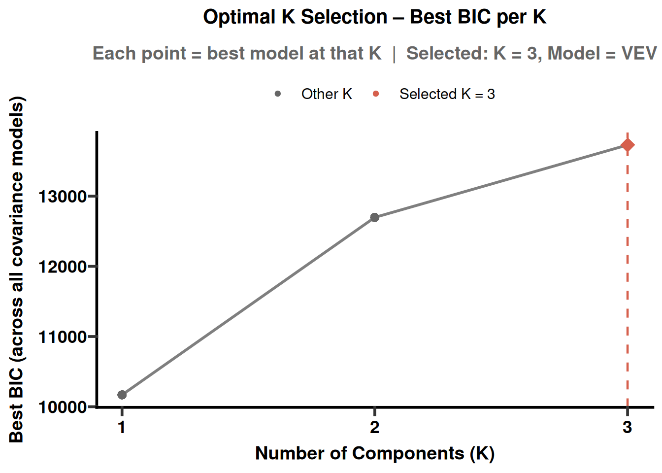
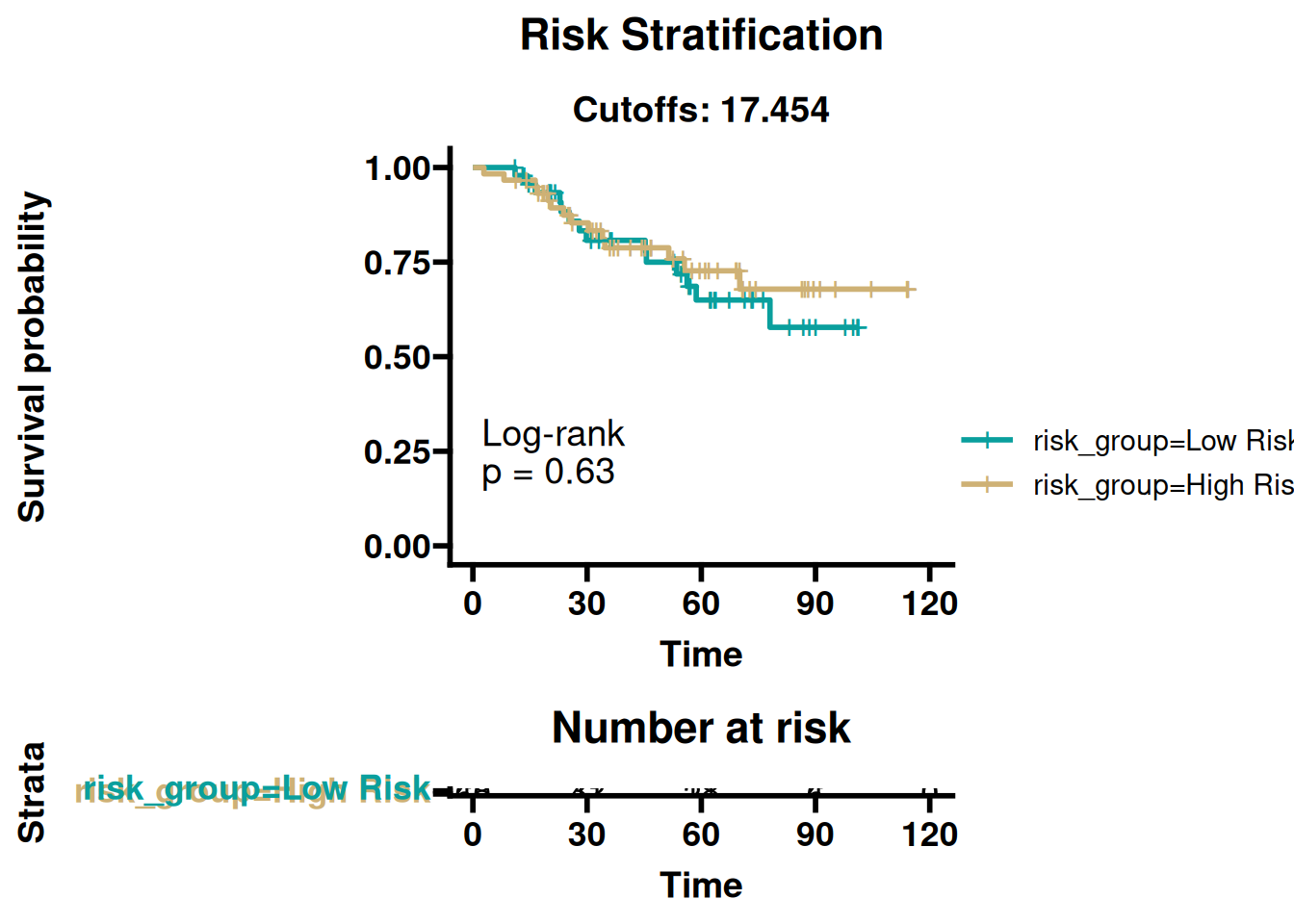
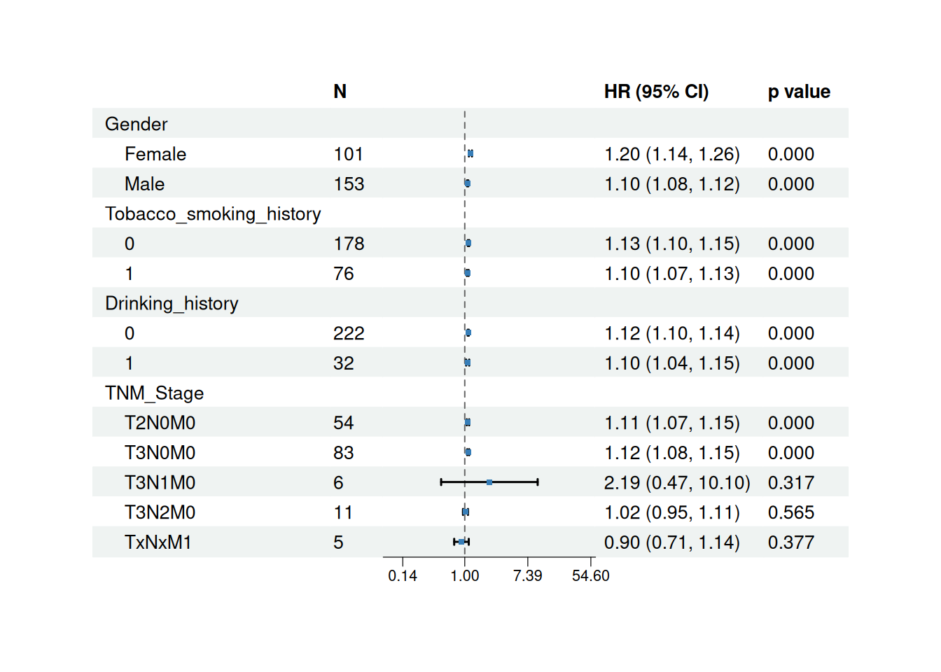
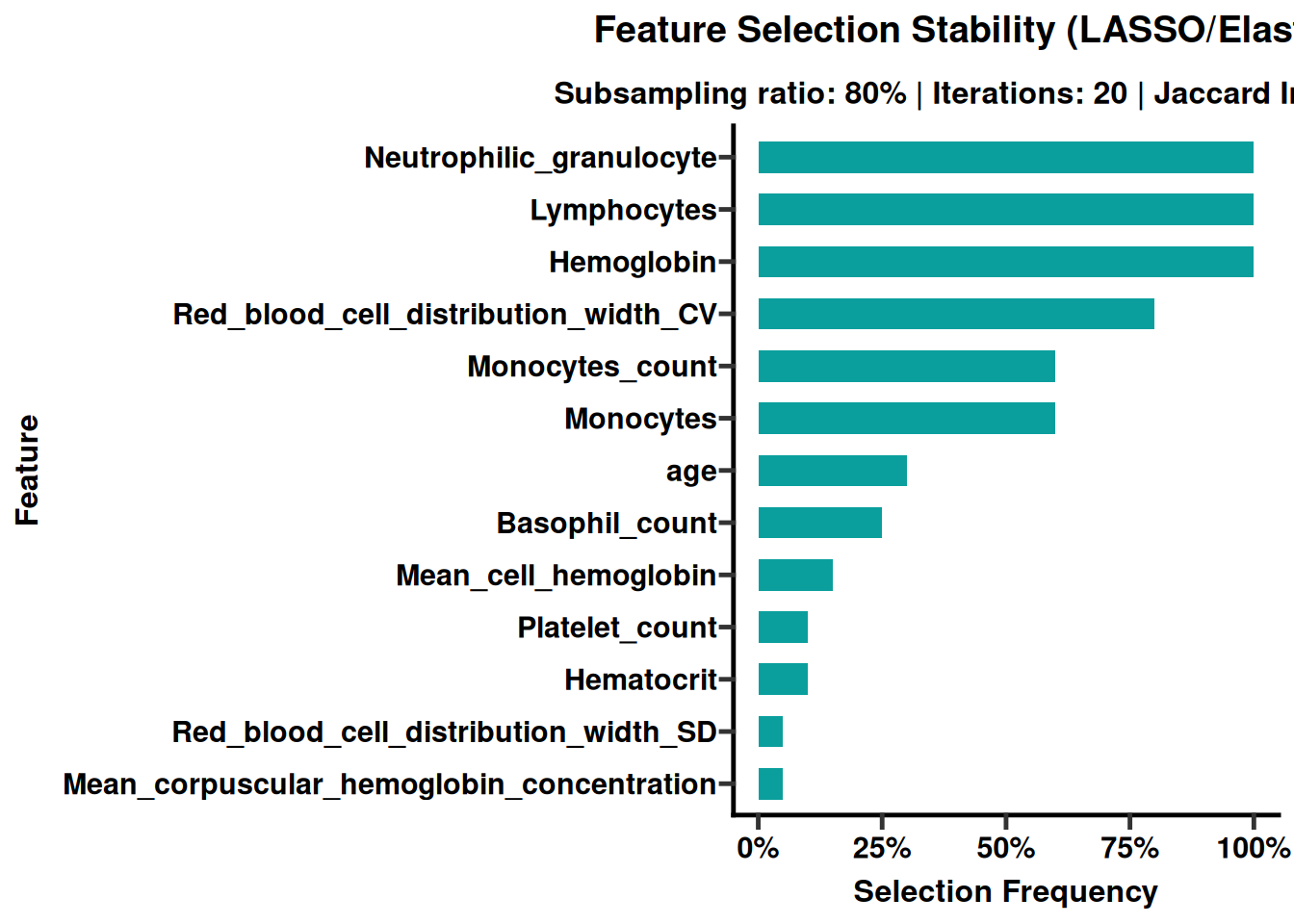
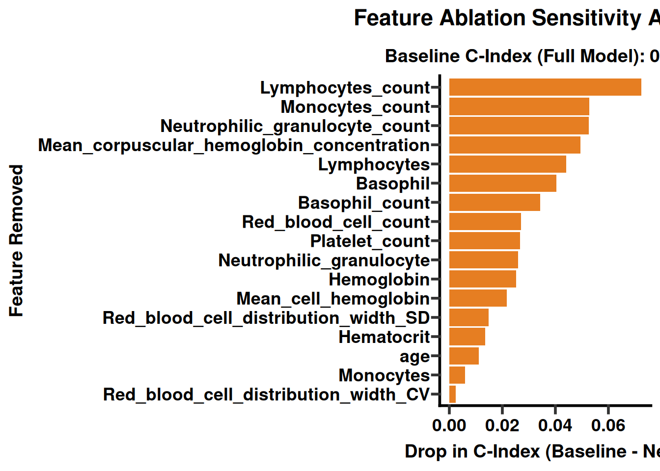
Every advanced script is designed to be run start-to-finish on your own cohort — swap in your data at the top of the CONFIG section and the rest of the pipeline (feature selection → modeling/clustering/survival → explainability → export) follows automatically.
# install.packages("remotes")
remotes::install_github("YuLab-SMU/icare", dependencies = TRUE)
icare depends on a large number of Bioconductor/CRAN packages (caret,
mlr3 + mlr3proba/mlr3tuning, survival, NMF, mclust, DALEX,
ComplexHeatmap, shiny, …) — see DESCRIPTION for the full list. A
plain remotes::install_github() will pull in the required CRAN
dependencies; Bioconductor packages (e.g. ComplexHeatmap) may need to be
installed separately first with BiocManager::install().
| # | Module | S4 object | What it does |
|---|---|---|---|
| 1 | Data cleaning | Stat |
Type detection, missing-value imputation, outlier handling, one-hot encoding, normalization, differential-feature testing, baseline ("Table 1") reports |
| 2 | Modeling | Train_Model |
Feature selection (RFE/GA/SA/built-in importance), train/test split, multi-algorithm benchmarking via caret, ensembling, hyperparameter tuning, SHAP/DALEX explainability, clinical thresholds & NRI/IDI |
| 3 | Subtyping | Subtyping |
Unsupervised clustering (K-means, NMF, latent profile analysis), cluster validation & cross-method agreement, marker-feature discovery, t-SNE/UMAP visualization |
| 4 | Survival / Prognosis | PrognosiX |
Cox / random-survival-forest / other mlr3proba learners, univariate + LASSO feature selection, risk stratification & KM curves, nomograms, decision-curve analysis |
Each module ships with a QUICKSTART vignette (minimal, sensible
defaults) and an ADVANCED vignette (every option, publication-style
figures) under vignettes/ — start there for runnable, end-to-end
examples on real data. The same chapters are also published as a
browsable book at yulab-smu.top/icare.
The tables below are a fast reference for the functions you'll use most
often in each module, grouped the way you'd actually call them in a
script. They mirror the shape of a normal icare analysis — see the
Quick start section for a compact end-to-end example, and
the vignettes for fully worked ones.
# Build the container ---------------------------------------------------
stat_obj <- CreateStatObject(raw.data = mat, info.data = inf,
                              group_col = "group", na.action = "allow")

# Clean it, one step per line -------------------------------------------
stat_obj <- stat_diagnose_variable_type(stat_obj)      # detect numeric vs. categorical
stat_obj <- stat_convert_variables(stat_obj)           # apply those types
stat_obj <- stat_miss_processed(stat_obj, impute_method = "median_mode")  # impute
stat_obj <- stat_detect_and_mark_outliers(stat_obj, method = "iqr")      # flag outliers
stat_obj <- stat_handle_outliers(stat_obj, method = "impute")            # fix them
stat_obj <- stat_onehot_encode(stat_obj)               # encode categoricals
stat_obj <- stat_normalize_process(stat_obj, method = "auto")            # normalize

# Explore & compare groups -----------------------------------------------
PlotGroupedDistribution(stat_obj, features = numeric_vars, group_col = "group")
PlotPCA(stat_obj, color_by = "group", ellipse = TRUE)
stat_obj    <- stat_var_feature(stat_obj, p_threshold = 0.05)   # differential features
deg_result  <- ExtractLastTestSig(stat_obj)
stat_obj    <- stat_gaze_analysis(stat_obj, save_word = TRUE)   # baseline "Table 1"

# Hand off to Module 2 / 3 ------------------------------------------------
saveRDS(stat_obj, "stat_obj.rds")| Command | Purpose |
|---|---|
CreateStatObject() |
Wrap a raw data matrix + metadata into a Stat object |
InspectObject() |
Print a structured summary of any icare S4 object |
stat_diagnose_variable_type() / stat_convert_variables() |
Detect and coerce numeric vs. categorical columns |
stat_miss_processed() |
Impute missing values ("median_mode", "mice", "knn", …) |
stat_detect_and_mark_outliers() / stat_handle_outliers() |
Flag and remediate outliers (IQR, Z-score, …) |
stat_onehot_encode() |
One-hot encode categorical variables |
stat_normalize_process() |
Normalize numeric variables ("auto", "z_score", "min_max", …) |
stat_var_feature() / batch_Wilcoxon() / ExtractLastTestSig() |
Univariate group-difference testing (differential features) |
stat_gaze_analysis() |
Publication-style baseline characteristics table |
PlotGroupedDistribution(), PlotPCA() |
Quick group-comparison and ordination plots |
# Convert & select features -----------------------------------------------
model_obj <- ConvertObject(stat_obj, to = "Train_Model")
builtin   <- FeatureSelectBuiltin(model_obj, models = c("rf", "glm"), top_n = 15)
model_obj <- ApplyFeatureSelection(model_obj, builtin$importance_table$Feature)

# Split + scale (fit on train, apply to test — no leakage) ----------------
idx <- caret::createDataPartition(model_obj@clean.df[[model_obj@group_col]], p = 0.7, list = FALSE)
model_obj@split.data <- list(training = model_obj@clean.df[idx, ],
                              testing  = model_obj@clean.df[-idx, ])
preProc <- caret::preProcess(model_obj@split.data$training, method = c("center", "scale"))
model_obj@split.scale.data <- list(training = predict(preProc, model_obj@split.data$training),
                                    testing  = predict(preProc, model_obj@split.data$testing))
model_obj@filtered.set <- model_obj@split.scale.data

# Train, compare, ensemble, tune -------------------------------------------
model_obj <- ModelTrainAnalysis(model_obj, methods = c("glmnet", "rf", "gbm"))
model_obj <- SelectBestModel(model_obj, metric = "auc")
model_obj <- TrainEnsemble(model_obj, strategy = "stacking", top_n = 4)
model_obj <- FineTuneModel(model_obj, method = "rf", bounds = BuildTuningBounds(mtry = c(2, 15)))

# Explain & apply clinically -----------------------------------------------
explainer <- CreateExplainer(model_obj)
ExplainSHAPBeeswarm(explainer)
thresh <- CalculateThresholds(model_obj, target_ppv = 0.9)

# Deploy ---------------------------------------------------------------------
deploy_manager <- ModelDeployment(model_obj, preproc = preProc,
                                   class_labels = c("Negative", "Positive"))
deploy_clinlab_app(deploy_manager)| Command | Purpose |
|---|---|
ConvertObject(x, to = "Train_Model") |
Turn a cleaned Stat object into a modeling object |
FeatureSelectBuiltin() / FeatureSelectionPipeline() (ga/rfe/sa) / run_feature_elimination() |
Feature selection: built-in importance, GA/RFE/SA, or performance-elbow elimination |
ApplyFeatureSelection() |
Commit to a final feature set |
PreprocessingBenchmark() / LogisticDiagnosticBenchmark() |
Compare imputation × normalization × algorithm combinations by CV performance |
ModelTrainAnalysis() |
Train and cross-validate multiple caret algorithms at once |
SelectBestModel() |
Pick the top-performing trained model |
TrainEnsemble() |
Combine models: "stacking", "average", "weighted", "voting" |
FineTuneModel() + BuildTuningBounds() / InspectHyperParams() |
Bayesian hyperparameter search around a chosen algorithm |
CreateExplainer() + ExplainSHAP*() / ExplainVariableImportance() / ExplainPartialDependence() |
DALEX/SHAP-based model explainability |
CalculateThresholds() / ApplyThreshold() / ClinicalThreshold() |
PPV/NPV/Youden decision thresholds |
ClinicalCorrelation() / PlotSubgroupForest() / PlotConfounderForest() |
Clinical covariate correlation, subgroup and confounder-adjusted forest plots |
CalculateCategoryNRI() / PlotIDICurve() / NRI_IDI_Analysis() |
Reclassification analysis (NRI/IDI) between two models |
PlotMultiROC(), PlotConfusionMatrix(), PlotCalibration(), PlotFeatureImportance() |
Standard performance visualizations |
ModelDeployment() + deploy_clinlab_app() |
Wrap trained model(s) + preprocessing into a predict function and Shiny app |
# Convert & normalize (min-max keeps values non-negative, required by NMF) --
sub_obj <- ConvertObject(stat_obj, to = "Subtyping")
sub_obj <- Sub_normalize_process(sub_obj, normalize_method = "min_max", group_col = "group")
sub_obj@scale.data <- remove_constant_columns(sub_obj@scale.data)

# Cluster: NMF (primary; produces a re-usable model) -------------------------
sub_obj <- Sub_nmf_estimate(sub_obj, rank_range = 2:6, nrun = 5, method = "brunet")
sub_obj <- Sub_nmf_best_rank(sub_obj, nrun = 5, method = "brunet")
sub_obj <- Sub_nmf_assign_subtypes(sub_obj)

# ... or K-means / LPA, and cross-compare -------------------------------------
sub_obj <- Sub_kmeans_with_optimal_k(sub_obj, k.max = 8)
sub_obj <- Sub_lpa_with_optimal_k(sub_obj, max_clusters = 3)
compare_clusterings(sub_obj, methods = c("cluster_kmeans", "cluster_lpa", "cluster_nmf"))

# Visualize, validate, find markers --------------------------------------------
sub_obj <- Sub_tsne_analyse(sub_obj, use_scaled_data = TRUE)
PlotDimReduction(sub_obj, reduction = "tsne", color_by = "cluster_nmf")
eval_result <- Sub_evaluation_results(sub_obj)
multi_deg   <- batch_Wilcoxon_MultiClass(mat = deg_df, group_col = "subtype")
PlotClusterHeatmap(sub_obj, deg_df = multi_deg, group_by = "cluster_nmf", top_n = 5)

# Deploy ------------------------------------------------------------------------
sub_manager <- New_Sub_Manager(sub_obj)
launch_sub_deploy_app(sub_manager)| Command | Purpose |
|---|---|
ConvertObject(x, to = "Subtyping") |
Turn a cleaned Stat object into a subtyping object |
Sub_normalize_process() / Sub_extract_norm_params() / Sub_apply_norm_params() |
Fit normalization on training data and replay it on validation/new data |
SplitSubtypingObject() |
Stratified train/validation split for cluster validation |
Sub_kmeans_with_optimal_k() |
K-means with automatic k selection |
Sub_lpa_with_optimal_k() |
Latent profile analysis (Gaussian mixture) |
Sub_nmf_estimate() → Sub_nmf_best_rank() → Sub_nmf_assign_subtypes() → Sub_nmf_train_model() |
Non-negative matrix factorization pipeline, including a re-usable model |
Sub_predict_subtypes() |
Assign new/validation samples to existing subtypes |
Sub_tsne_analyse() / Sub_umap_analyse() + PlotDimReduction() |
Dimensionality reduction for visualization |
Sub_evaluation_results() |
Cluster-quality metrics (silhouette, etc.) |
compare_clusterings() / plot_clustering_comparison() |
Adjusted Rand Index agreement between methods |
batch_Wilcoxon_MultiClass() + PlotClusterHeatmap() / PlotGroupMeanHeatmap() |
Subtype-specific marker discovery and heatmaps |
PlotSilhouette() / PlotMultiAlluvial() |
Separation diagnostics and multi-method/outcome alluvial plots |
New_Sub_Manager() + launch_sub_deploy_app() |
Deploy the trained subtyping model as a Shiny app |
# Convert (moves time/status into info.data, keeps numeric features) --------
stat <- CreateStatObject(raw.data = df, group_col = NULL, na.action = "allow")
prog <- Stat_to_PrognosiX(stat, time_col = "time", status_col = "status", min_events = 10)

# Feature selection: univariate Cox + LASSO -----------------------------------
feat_sel <- surv_feature_selection_multi(prog, methods = c("uni_cox", "lasso"), combine = "union")
prog@survival.var <- list(selected = feat_sel$selected)

# Train/validation split (mlr3 tasks) ------------------------------------------
task <- surv_extract_task(prog)$select(feat_sel$selected)
train_task <- task$clone()$filter(train_idx)
val_task   <- task$clone()$filter(val_idx)

# Benchmark algorithms, then train and tune the winner --------------------------
bmr   <- surv_run_algorithm_benchmark(train_task, learners_list = c("surv.coxph", "surv.ranger"))
learner <- surv_get_learner("surv.ranger", train_task)
learner$train(train_task)
tuned   <- surv_train_and_tune(train_task, "surv.ranger")

# Evaluate, stratify risk, and validate -----------------------------------------
surv_evaluate_model(learner, val_task)
km <- surv_plot_risk_km(learner, train_task, cutoff_method = "median", risk_table = TRUE)
nom <- surv_generate_nomogram(prog, features = feat_sel$selected)   # includes a PH check

# Predict for new patients and deploy ---------------------------------------------
predict_prognosix(prog, new_patients)
predict_risk_groups(prog, new_patients, cutoff_method = "median")
prog_manager <- New_Prog_Manager(prog)
launch_prog_deploy_app(prog_manager)| Command | Purpose |
|---|---|
Stat_to_PrognosiX() |
Convert a Stat object into a survival-modeling (PrognosiX) object |
surv_feature_selection_multi() |
Univariate Cox / LASSO feature selection (combine = "union"/"intersect") |
surv_extract_task() |
Build an mlr3proba::TaskSurv from a PrognosiX object |
surv_get_learner() / surv_run_algorithm_benchmark() |
Instantiate or cross-validate mlr3proba survival learners (Cox, RSF, surv.ranger, …) |
surv_train_and_tune() |
Hyperparameter tuning of a survival learner |
surv_evaluate_model() |
C-index / Brier score / time-dependent AUC evaluation |
surv_plot_risk_km() |
Kaplan–Meier risk stratification ("median", "tertile", "quartile", "p_optimize", "custom") |
surv_generate_nomogram() |
Cox-based nomogram, with an automatic proportional-hazards (cox.zph) check |
predict_prognosix() / predict_risk_groups() |
Score and risk-classify new patients |
run_prognosis_pipeline() |
End-to-end orchestration of the steps above in one call |
New_Prog_Manager() + launch_prog_deploy_app() |
Deploy the trained survival model as a Shiny app |
Methodological note. Several of the "essential commands" above only
report an unbiased estimate of performance when you actually pass a
held-out split (val_task,split.data$testing, …) rather than
re-using the data a model was trained/tuned on — e.g.surv_plot_risk_km()
andsurv_generate_nomogram()will happily run on the training task, but
the resulting p-values/HRs should then be treated as descriptive, not
confirmatory. See each function's documentation for details.
For package versions that include the tutorial dataset, its source location is icare/inst/extdata/PMID37633276_DIA_plasmaproomic.xlsx; after installation, locate it with system.file("extdata", "PMID37633276_DIA_plasmaproomic.xlsx", package = "icare") (an empty string means the installed version does not include the file).
The fastest way to see the whole pipeline end-to-end is the QUICKSTART
vignette for each module, in order:
library(icare)

# Module 1: raw data -> cleaned Stat object -> stat_obj.rds
source(system.file("vignettes", "01_module1_data_cleaning_QUICKSTART.R", package = "icare"))

# Module 2: stat_obj.rds -> trained/evaluated Train_Model -> model_obj.rds
source(system.file("vignettes", "02_module2_modeling_QUICKSTART.R", package = "icare"))

# Module 3: stat_obj.rds -> NMF subtypes -> subtyping_obj.rds
source(system.file("vignettes", "03_module3_subtyping_QUICKSTART.R", package = "icare"))

# Module 4: your own time/status data.frame -> survival model + KM/risk groups
source(system.file("vignettes", "04_module4_survival_QUICKSTART.R", package = "icare"))
Each QUICKSTART script points to its ADVANCED counterpart for the full
option set (multi-method feature selection, ensembling, tuning,
SHAP/DALEX explanations, clinical thresholds & NRI/IDI, cluster
cross-validation, survival benchmarking, decision-curve analysis, and
the Shiny deployment apps). Prefer to read rather than run? The same
scripts are rendered with output and figures at
yulab-smu.top/icare.
- Full documentation & worked examples: yulab-smu.top/icare
- Function-level help:
?FunctionNameinside R, orInspectObject(x)to
inspect any icare S4 object's current state. - Bug reports and feature requests: please open a
GitHub issue with a minimal reproducible example.
Huaichao Luo, Fei Long, Hongyan Lin, Xin Li, Ruohao Wu, Jixue Wang, Chunhui Yuan, Xingmei Zhang, Xiaohui Wang, Dongsheng Wang, Yang Luo, Weiyan Zhou, Fubing Wang, Jian Huang, Guangchuang Yu. icare: Intelligent ClinlAbomics Research Expedition. R package version 1.1.0GPL-3 © Huaichao Luo, Fei Long, Hongyan Lin, Jian Huang, Guangchuang Yu